Description
The irisws-timeseries service provides access to individual channels of time series data for a specified time range. Requested segments may be up to 30 days in length and optional signal processing may be applied to return data. The time series may be returned in a variety of formats.
Output format options:
- miniSEED
- SAC zip (binary little endian)
SAC Alpha(ASCII) [deprecated]SAC binary(big & little endian) [deprecated]- Audio (WAV format)
- PNG Plot
- ASCII (data column)
- ASCII (data column, time column)
- GEOCSV (data column)
- GEOCSV (data column, time column)
Signal processing options (operations are performed in the order specified):
- high, low and band-pass filter
- remove mean value
- scaling by constant value
- deconvolution of instrument response (with frequency limits and unit conversion)
- differentiation and integration
- decimation to lower sample rates
Contents
- Digital Signal Processing
- Audio Output
- Plot Output
- URL Builer
- Invoking from the UNIX command line
- Data length limitations
- Accessing Restricted Data
Digital Signal Processing
There are 15 digital signal processing parameter options.
- taper
- envelope
- hpfilter
- lpfilter
- bpfilter
- demean
- scale
- divscale
- correct
- autolimits
- freqlimits
- units
- diff
- int
- deci
Parameter Order Matters!
For the digital signal processing parameters lpfilter, hpfilter, bpfilter, demean, diff, int, units and deci the order in which they are listed as query parameters can matter. The ws-timeseries web service will apply the operations in the order in which they are listed reading left to right. For example, applying demean before correct rather than after can yield dramatically different results:
http://service.iris.edu/irisws/timeseries/1/query?net=IU&sta=ANMO&loc=00&cha=BHZ&starttime=2010-02-27T06:30:00&endtime=2010-02-27T10:30:00&demean=true&correct=true&output=plot
versus:
http://service.iris.edu/irisws/timeseries/1/query?net=IU&sta=ANMO&loc=00&cha=BHZ&starttime=2010-02-27T06:30:00&endtime=2010-02-27T10:30:00&correct=true&demean=true&output=plot
Note: the URL Builder does not allow the order of parameters to be adjusted. However, the order of parameters that it presents should, in general, be useful.
taper
The taper option applies a symmetric tapering function, sometimes called a window function, to the time series data. The specified width is given as a fraction of the total width and must be in the range 0-0.5. The taper option is typically used to remove end-effects. It should be be specified before other filtering options (See Parameter Order Matters! below).
For example, if a value of 0.25 is given and the time series is 100 seconds long, the first 25 seconds of data will be multiplied by a value ranging from 0 (time=0 seconds) to 1 (time=25 seconds), from 25 seconds to 75 seconds, the data will be unaltered and for the last 25 seconds the data will be multiplied by a value ranging from 1 (time=75 seconds) to 0 (time=100 seconds).
Supported taper functions are HANNING, COSINE and HAMMING. If a taper function name is not specified, the HANNING function is used. Examples:
taper=0.5 — Hanning taper function that varies over full width
taper=0.5,HANNING — Same as previous
taper=0.25,COSINE — Cosine with tapers on first and last quarters, flat over middle half
taper=0.333,HAMMING — Hamming with tapers on first and last thirds, flat over middle third
envelope
The envelope calculates the envelope of the time series using a Hilbert transform approximated by a time domain filter.
hpfilter, lpfilter, bpfilter
The hpfilter (high-pass), lpfilter (low-pass) and bpfilter (band-pass) options apply 4-pole, 2-pass Butterworth filters to the data. The options take numeric values of cycles per second (hertz). For bpfilter two frequencies must be given. These two values may be separated by any of [-,/;]. For example, the following are equivalent:
bpfilter=0.001-0.01
bpfilter=0.001,0.01
bpfilter=0.001/0.01
bpfilter=0.001;0.01
These filtering options operations retain the original DC offset by removing the mean value prior to filtering and then restoring the mean value upon completion.
demean
The demean option removes mean value from the digital signal. This option is usually applied first (See Parameter Order Matters! below).
scale, divscale
The scale option multiplies the digital signal by the specified value. If scale=AUTO is given, the data samples are scaled by the the total sensitivity defined in the metadata for the channel (SEED response stage-zero gain). The divscale option divides each data sample by the specified value. Both scale=AUTO and correct cannot be specified.
correct, autolimits, freqlimits, units
The correct option removes the instrument response from the signal using the current instrument response metadata in the DMC’s database unless that metadata contains a stage zero polynomial response correction in which case that is applied to the signal. Polynomial responses are commonly associated with temperature and pressure sensor data.
freqlimits
The freqlimits option applies both a low-pass and high-pass taper (in the frequency domain). The option can only be used if the correct option is also given. Four frequencies are given in cycles per second (Hertz). The values may be separated by any of [-,/;]. For example, the following are equivalent:
freqlimits=0.0033-0.004-0.05-0.06
freqlimits=0.0033,0.004,0.05,0.06
freqlimits=0.0033/0.004/0.05/0.06
freqlimits=0.0033;0.004;0.05;0.06
autolimits
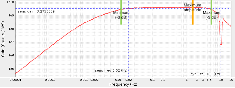
The autolimits option automatically determines the “flat” band of the amplitude response and sets the frequency limits that would otherwise be specified using the freqlimits option. A decibel drop (dBdown) value for both the upper and lower limits is specified and used to determine the frequency range of the passband. It is mutually exclusive with the freqlimits option and can only be specified if the correct option is also given.
The algorithm is designed to find a flat pass band in the units requested such as requesting output in velocity for an sensor flat to velocity. Other combinations will likely result in unsatisfactory results, i.e. requesting output in displacement for a sensor flat to velocity.
How autolimits determines the passband
The upper and lower frequency limits are identified by searching the response for amplitude values that are a specified number of decibels lower than the maximum amplitude. The maximum amplitude is usually within the flat portion of passband.

units
The units option allows for requesting units to be to displacement, velocity, or acceleration:
units=DIS
units=VEL
units=ACC
units=DEF — default units specified by the response metadata
The units option can only be used if the correct option is also given.
Description
diff, int
The diff option differentiates the data using the 2-point (uncentered ) method. The int option integrates the data using the trapezoidal (midpoint) method.
deci
The deci option decimates the signal to the given cycles per second (hertz) sample rate. The actual output sample rate may differ from the selected sample rate. The service will use the closest output rate such that the ratio of the source rate to output rate is factorable by the numbers 2,3,5 and 7. For example, if the selected data is sampled at 50 Hz and deci=3.0 is selected, the output data will have a sample rate of 3.125 Hz as this is the closest achievable sample rate. This is illustrated in the following table which shows sample rates which can be decimated to from data sampled at 50 Hz going out to 2.0 Hz
50.0/2   [2]          = 25.000000
50.0/3   [3]          = 16.666667
50.0/4   [2x2]        = 12.500000
50.0/5   [5]          = 10.000000
50.0/6   [2x3]        = 8.333333
50.0/7   [7]          = 7.142857
50.0/8   [2x2x2]      = 6.250000
50.0/9   [3x3]        = 5.555556
50.0/10  [2x5]        = 5.000000
50.0/12  [2x2x3]      = 4.166667
50.0/14  [2x7]        = 3.571429
50.0/15  [3x5]        = 3.333333
50.0/16  [2x2x2x2]    = 3.125000 <<< closest value to 3.0 Hz
50.0/18  [2x3x3]      = 2.777778
50.0/20  [2x2x5]      = 2.500000
50.0/21  [3x7]        = 2.380952
50.0/24  [2x2x2x3]    = 2.083333
50.0/25  [5x5]        = 2.000000
A linear-phase, lowpass filter is applied to the data as an anti-aliasing filter in the decimation process.
Comparison to SAC
The digital signal processing algorithms used by ws-timeseries are similar to the those used by the SAC (Seismic Analysis Code) software package.
| ws-timeseries parameter | equivalent SAC Command |
|---|---|
lpfilter |
LOWPASS |
hpfilter |
HIGHPASS |
bpfilter |
BANDPASS |
demean |
RMEAN |
diff |
DIF |
int |
INT |
correct |
TRANSFER |
freqlimits |
TRANSFER (FREQlimits) |
units |
TRANSFER (TO +NONE, +ACC, +VEL) |
decimate |
DECIMATE |
The lpfilter, hpfilter and bpfilter operators are analogous to the SAC LOWPASS, HIGHPASS and BANDPASS commands. ws-timeseries uses 4-pole, 2-pass Butterworth filters.
The deci option is different than the SAC DECIMATE option in that you specify the sample rate to decimate down to. The algorithm used is the same as used by SAC. It requires that the output sample-rate divided by the source sample-sample rate be factorable by 2,3,5 and 7.
The freqlimits parameter can only be used with the correct option. It is analogous to FREQlimits used by the SAC TRANSFER command. The freqlimits describe the shape of a frequency domain taper window. The taper window is applied to the data after being transfered to the frequency domain during the deconvolution operation.
Audio Output
With the output=audio option ws-timeseries can produce WAV audio files. There are two related options available: audiosamplerate and audiocompress. The audiosample parameter will cause the audio output to be played at the given rate. The audiocompress option will apply dynamic gain adjustment that tends to equalize the volume level of loud periods of time relative to quite periods of time.
Programs such as Amadeus and Audacity can be useful for listening to and adjusting the audio output from ws-timeseries. Both of these programs allow the audio sample-rate and audio-compression to be quickly adjusted. Rather than repeatedly calling ws-timeseries with different sample-rates, it may be more useful to download a section of data and adjust the sample rate locally to hear differences in the sound.
The web page http://geophysics.eas.gatech.edu/people/zpeng/EQ_Music/ by Zhigang Peng of the Georgia Institute of Technology contains more information about the sonification of earthquake data.
Plot Output
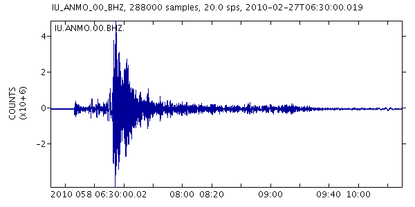
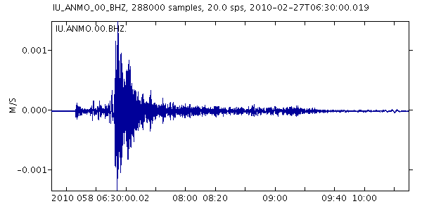
With the output=plot option ws-timeseries can produce simple plots of seismic data. With the minimum options (net, sta, loc, cha, start and end) ws-timeseries will produce plots with units of “COUNTS”. With the scale=AUTO or correct options meaningful units will be applied to the plots. For example:
http://service.iris.edu/irisws/timeseries/1/query?net=IU&sta=ANMO&loc=00&cha=BHZ&starttime=2010-02-27T06:30:00&endtime=2010-02-27T10:30:00&output=plot&width=600&height=300

http://service.iris.edu/irisws/timeseries/1/query?scale=AUTO&net=IU&sta=ANMO&loc=00&cha=BHZ&starttime=2010-02-27T06:30:00&endtime=2010-02-27T10:30:00&output=plot&width=600&height=300

The plot dimension options width and height can be used to produce larger or smaller plots. The combined product of width times height must be less than 6,000,000.
The antialias option will produce plots with a less jagged appearance. Using this option can increase the amount of time needed to generate the plot and may cause failures for large data sets.
URL Builder
The easiest way to gain an understanding of how to use ws-timeseries is by experimenting with its URL builder. This web page makes it relatively easy to understand what combinations of query parameters are legal for this web service. The web page will dynamically activate and deactivate different options as you make selections. For example, if the output is set to audio, then “Audio Dynamic Range Compression” and “Audio Sample Rate” become available for selection. The URL at the bottom of the page shows what the URL for the request will look like. Clicking the URL will cause the request to be sent to the server.
Data length limitations
The longest length of data that can be requested with ws-timeseries is 31 days. If you are interested in longer intervals, please consider using fdsnws-dataselect. In general, requesting data with a large number of samples can be problematical for this web service. Data filtering, plotting and audio conversion may fail if too many samples exist in the time window. How the service will fail is not completely deterministic. For example, large requests can cause network timeouts which may depend on how your client reaches the IRIS web servers. In general, requesting data windows that are less than a day long should work without difficulty. For any given time window, low sample rate channels (for example LHZ), will be less likely to cause failure than high sample rate channels (for example EHZ).
See also: http://www.iris.washington.edu/manuals/SEED_appA.htm.
Invoking from the UNIX command line
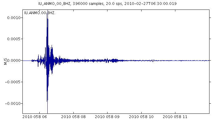
ws-timeseries can be easily invoked using the UNIX wget and curl commands. The following demonstrates using wget to download a plot of filtered data.
$ wget —content-disposition “http://service.iris.edu/irisws/timeseries/1/query?net=IU&sta=ANMO&loc=00&cha=BHZ&starttime=2010-02-27T06.30.00&endtime=2010-02-27T12.00.00&demean=true&scale=AUTO&lpfilter=0.05&width=700&height=400&output=plot”
Resolving service.iris.edu…
Connecting to service.iris.edu|…|:80… connected.
HTTP request sent, awaiting response… 200 OK
Length: 4198 (4.1K) [image/png]
Saving to: ‘ANMO.IU.00.BHZ.2010.058.06.30.00.019-2010.058.11.59.59.969.lp-0.05.rm.scale-AUTO.png’100%[=========================================>] 4,198 —.-K/s in 0s
2012-01-01 15:15:03 (200 MB/s) – ‘ANMO.IU.00.BHZ.2010.058.06.30.00.019-2010.058.11.59.59.969.lp-0.05.rm.scale-AUTO.png’ saved [4198/4198]

Because of the ampersand (&) characters in the URL, the URL must be surrounded by quote characters (”“) or the UNIX shell will interpret them as background control characters. The --content-disposition flag tells wget to save the file to the name indicated in the HTTP response header. This file name is automatically generated by the web service.
In the previous example the auto-generated name was:
ANMO.IU.00.BHZ.2010.058.06.30.00.019-2010.058.11.59.59.969.lp-0.05.rm.scale-AUTO.png
The --content-disposition flag is only available in more recent versions of wget. To save to a file of your own choosing, use the -O option.
Accessing Restricted Data
Requesting restricted data via this web service requires authentication. The authentication is done using a standard HTTP mechanism called digest access authentication, a sort of 3-way handshake. To submit a request with authentication credentials you would use the queryauth method of the service in place of the query method. You must use client that supports digest authentication, luckily such support is common.
For example, submitting a request and initiating the authentication handshake would be done by requesting this URL:
http://service.iris.edu/irisws/timeseries/1/queryauth?net=IU&sta=ANMO&loc=00&cha=BHZ&start=2010-02-27T06:30:00&end=2010-02-27T10:30:00&output=plot
This request could be submitted and using a command line tool like curl:
$ curl -L --digest --user EMAIL:PASSWORD -o plot.png 'http://service.iris.edu/irisws/timeseries/1/queryauth?net=IU&sta=ANMO&loc=00&cha=BHZ&start=2010-02-27T06:30:00&end=2010-02-27T10:30:00&output=plot'
where you replace EMAIL and PASSWORD with your own credentials.
You may test your software with the test credentials: email=nobody@iris.edu and password=anonymous. A working version of the curl example above using the test credentials:
$ curl -L --digest --user nobody@iris.edu:anonymous -o plot.png 'http://service.iris.edu/irisws/timeseries/1/queryauth?net=IU&sta=ANMO&loc=00&cha=BHZ&start=2010-02-27T06:30:00&end=2010-02-27T10:30:00&output=plot'
We recommend always using the -L option to allow curl to follow HTTP redirections specified by our systems. The DMC uses HTTP redirection during maintenance to keep servicing requests.
See also:
- http://www.gnu.org/software/wget/manual/wget.html
- http://curl.haxx.se/
- http://en.wikipedia.org/wiki/List_of_HTTP_header_fields#Responses
- http://en.wikipedia.org/wiki/MIME#Content-Disposition
Problems with this service?
Please send an email report of which service you were using, your URL query, and any error feedback to:
data-help@earthscope.org
We will address your issue as soon as possible.

