Description
The noise-mode-timeseries web service returns Probability Density Function daily mode estimates for individual seismic channels measured at discrete frequencies as a function of time.
Contents
Introduction
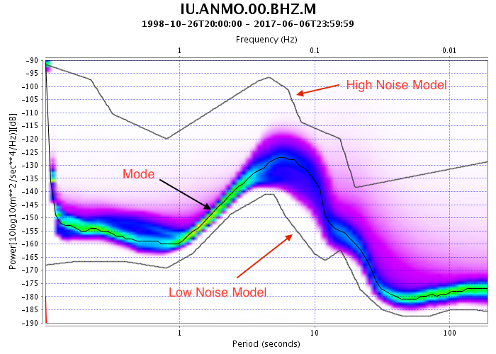
The Power Density Function (PDF) represents the distribution of noise power as a function of frequency. The PDF mode function represents the most commonly occurring (most likely) noise power level as a function of frequency.
The following plot, from the noise-pdf webservice, shows a computed PDF from 19 years of data from one seismometer along with the computed mode function.

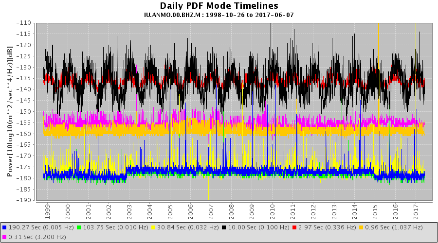
The noise-mode-timeseries web service reveals how the PDF mode function varies over time. It returns PDF mode estimates compiled from 24 hour windows with UTC day boundaries.
The following plot, from the noise-mode-timeseries web service, shows the daily PDF mode variations, measured at 7 frequencies, from the same data used to generate the previous PDF plot.

At periods of 10.0 and 2.97 seconds seasonal variations of noise level are clearly visible and at 190.27 and 103.75 seconds step level changes are also visible.
The daily PDF mode functions are computed at about 88 frequencies. It is generally not useful to plot this many timeseries in one plot. See “Frequency Selection” for details on how to customize the selection of frequencies.
The web service provides an output option that allows the PDF modes to be displayed relative to the Peterson noise models or relative to user defined noise models. See “Noise Model Comparison” for details.
Output Formats
The web service provides three output formats:
- plot – Generates plot images
- xml – Generates XML data documents
- text. – Generates text data documents
Plot Format
With the format=plot output option, the webservice returns PNG plots of the daily PDF modes.
Plot Customization
Fourteen options allow for customizing plot appearance.
Plot Dimensions
plot.width and plot.height allow for customizing the size of the generated plot images.
Example: 2000×1000 image.
Title Customization
plot.title and plot.subtitle options allow for customizing the plot titles. If the title or subtitle are hide, they will not be shown.
Example: No Subtitle and Title is ANMO 1998 – 2017 Daily PDF Modes
Tip: When setting the title, the character sequence %20 can be used for white spaces and %0A can be used for carriage-return. See Percent-encoding: Wikipedia for more information.
Domain Range
plot.power.min and plot.power.max options allow for customizing the domain of the generated plots. By default the range is auto selected. This can make comparing plots from different data sets difficult. These options make comparing plots easier. plot.power.min and plot.power.max must be specified together.
Example: Power range -185 to -115
Font Sizes
Font sizes can be set for six different aspects of the plot:
plot.titlefont.size– title on the topplot.subtitlefont.size– subtitleplot.powerlablefont.size– power axis titleplot.poweraxisfont.size– power axis labelsplot.timeaxisfont.size– time axis labelsplot.legendfont.size– legend at the bottom of the plot
Example: Time Axis Font size to 24
The plot.legend option is used for hiding the legend box at the bottom of the plot. Use plot.legend=hide to hide the legend and plot.legend=show to show (default).
Example: No Legend
XML Format
With the format=xml option the service produces XML documents useful for machine processing.
There are two options that effect XML formatting: xml.style and xml.units.
xml.style effects how output information is grouped:
xml.style=bydaydefault Group output by day. (example)xml.style=byfrequencyGroup output by frequencies. (example)xml.style=byperiodGroup output by periods. (example)xml.style=flatno grouping.(example)
xml.units effect whether period or frequency is output. This option is mainly useful with xml.style=byday and xml.style=flat.
xml.units=secondsShow results by period. (example)xml.units=hertzdefault Show results by frequency. (example)
Text Format
With the format=text option the service produces text documents useful for machine processing or human reading.
There are two options that effect text formatting text.style and text.units.
text.style effects how output information is grouped:
text.style=listdefault Group (list) of rows for each day. (example)text.style=tableSingle row for each day. (example)
text.units Effect whether period or frequency is output.
text.units=secondsShow results by period. (example)text.units=hertzdefault Show results by frequency. (example)
Noise Model Comparison
The output and noisemodel.byperiod and noisemodel.byfrequency options allow the mode power levels to be compared to noise models.
The web service contains default high and low noise models derived from tables 3 and 4 in Observations and Modeling of Seismic Background Noise by Jon Peterson, 1993.
The default noise models can be view from the link /defaultnoisemodel. Noise models are interpolated using a piecewise log, linear relationship given by:
Noise = A + B Log10(Period)
Noise model levels are interpreted as constant above and below model specifications.
output option
The output option accepts the following three values: power, powerdhnm, powerdlnm and powerdnm
output=power is the default. Output values are simply the mode power levels. (example)
output=powerdhnm: power values are differenced against the high-noise model. (example)
output=powerdlnm: power values are differenced against the low-noise model. (example)
output=powerdnm: power values are compared to both the high and low noise models. (example)
Power levels are returned with the following logic:
    if( power > HNM )
       return (power - HNM)
    else if ( power < LNM )
       return (power - LNM)
    else
       return 0
With output formats format=plot and format=text only one output parameter may be specified. However, when format=xml is specified, multiple values can be used.
Example: …format=xml&output=power,powerdhnm,powerdlnm,powerdnm
noisemodel.byperiod and noisemodel.byfrequency Options
The noisemodel.byperiod and noisemodel.byfrequency options allow for the input of custom noise models.
The noise model parameters accept both high and low noise models or a single noise model. If a single noise model is specified
the output options powerdhnm, powerdlnm, powerdnm will all return the same values.
The noise models should be in the format
High and low models by period:
noisemodel.byperiod=period1,valueA1,valueB1|period2,valueA2,valueB2|period3,valueA3,valueB3...
Single model by period:
noisemodel.byperiod=period1,value1|period2,value2|period3,value3...
High and low models by frequency:
noisemodel.byfreqeuncy=frequency1,valueA1,valueB1|frequency2,valueA2,valueB2|frequency3,valueA3,valueB3...
Single model by frequency:
noisemodel.byfreqeuncy=frequency1,value1|frequency2,value2|frequency3,value3...
For high/low models (two values per frequency or period) the order of the value pairs is not important; greater values are assigned to the high noise model and lower values are assigned to the low noise model. The order of frequencies (or periods) is not important; however, there should be no duplicates.
The character sequence %7C can be used in place of the | (pipe) character in URLs.
Example
Frequency and Period Selection
The mutually exclusive options frequencies and periods allow for choosing which frequencies or powers are selected for output.
Output values which are closest to the input values are selected. This alleviates the user from having to know the analyzed periods or frequencies exactly.
Default Selection
By default, the frequencies which are closest to the following set of frequencies are selected for output:
0.00001, 0.000032, 0.0001, 0.00032, 0.001, 0.0032, 0.01, 0.032, 0.1, 0.32, 1.0, 3.2, 10.0, 32.0, 100.0, 320.0 hertz
Selection by List
Frequencies or periods can be selected using a comma selected list:
Examples:
Selection by Range
Frequencies or periods can be selected by range using the notation
[start,end]
The start and end can be switched. For example, [1,2] and [2,1] will yield the same results.
Examples:
Tip: %5B can be substituted for the [ character and %5D can be substituted for the ] character in URLs
Selection of all available frequencies/periods
Use frequecies=all or periods=all to selection all available frequencies and periods
Example
…format=plot&frequencies=all
References
Wikipedia: Percent-encoding
Ambient Noise levels in the Continental United States
by Daniel E. McNamara and Raymond P. Buland
“Observations and Modeling of Seismic Background Noise”:
https://doi.org/10.3133/ofr93322 by Jon Peterson, 1993.
Problems with this service?
Please send an email report of which service you were using, your URL query, and any error feedback to:
data-help@earthscope.org
We will address your issue as soon as possible.

